Diversity estimation
Note
Application of routines from this section is described in the following tutorial.
PlotQuantileStats
Plots a three-layer donut chart to visualize the repertoire clonality.
- First layer (“set”) includes the frequency of singleton (“1”, met once), doubleton (“2”, met twice) and high-order (“3+”, met three or more times) clonotypes. Singleton and doubleton frequency is an important factor in estimating the total repertoire diversity, e.g. Chao1 diversity estimator (see Colwell et al). We have also recently shown that in whole blood samples, singletons have very nice correlation with the number of naive T-cells, which are the backbone of immune repertoire diversity.
- The second layer (“quantile”), displays the abundance of top 20% (“Q1”), next 20% (“Q2”), … (up to “Q5”) clonotypes for clonotypes from “3+” set. In our experience this quantile plot is a simple and efficient way to display repertoire clonality.
- The last layer (“top”) displays the individual abundances of top N clonotypes.
Command line usage
java -Xmx4G -jar vdjtools.jar PlotQuantileStats [options] sample.txt output_prefix
Parameters:
| Shorthand | Long name | Argument | Description |
|---|---|---|---|
-t |
--top |
int | Number of top clonotypes to visualize. Should not exceed 10, default is 5 |
-h |
--help |
Display help message |
Tabular output
Following table with .qstat.txt prefix is generated,
| Column | Description |
|---|---|
| Type | Detalization level: set, quantile or top |
| Name | Variable name: “1”, “Q1”, “CASSLAPGATNEKLFF”, etc |
| Value | Corresponding relative abundance |
Graphical output
Following plot with .qstat.pdf prefix is generated,
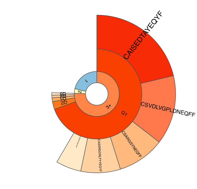
Sample clonality plot. See above for the description of plot structure.
RarefactionPlot
Plots rarefaction curves for specified list of samples, that is, the dependencies between sample diversity and sample size. Those curves are interpolated from 0 to the current sample size and then extrapolated up to the size of the largest of samples, allowing comparison of diversity estimates. Interpolation and extrapolation are based on multinomial models, see Colwell et al for details.
Command line usage
java -Xmx4G -jar vdjtools.jar RarefactionPlot \
[options] [sample1.txt sample2.txt ... if -m is not specified] output_prefix
Parameters
| Shorthand | Long name | Argument | Description |
|---|---|---|---|
-m |
--metadata |
path | Path to metadata file. See Common parameters |
-i |
--intersect-type |
string | Set the intersection type used to collapse clonotypes before computing diversity. Defaults to strict (don’t collapse at all). See Common parameters |
-s |
--steps |
integer | Set the total number of points in the rarefaction curve, default is 101 |
-f |
--factor |
string | Specifies plotting factor. See Common parameters |
-n |
--numeric |
Specifies if plotting factor is numeric. See Common parameters | |
-l |
--label |
string | Specifies label used for plotting. See Common parameters |
--wide-plot |
Set wide plotting area | ||
--label-exact |
If set to true, will position sample labels exactly at observed samle size, will use the extrapolated sample size otherwise | ||
-h |
--help |
Display help message |
Tabular output
The following table with
rarefaction.[intersection type shorthand].txt is generated:
| Column | Definition |
|---|---|
| sample_id | Sample unique identifier |
| … | Sample metadata columns, see Metadata section |
| x | Subsample size, reads |
| mean | Mean diversity at given size |
| ciL | Lower bound of 95% confidence interval |
| ciU | Upper bound of 95% confidence interval |
| type | Data point type: 0=interpolation, 1=exact, 2=extrapolation |
Graphical output
A figure with the same suffix as output table and .pdf extension is
provided.
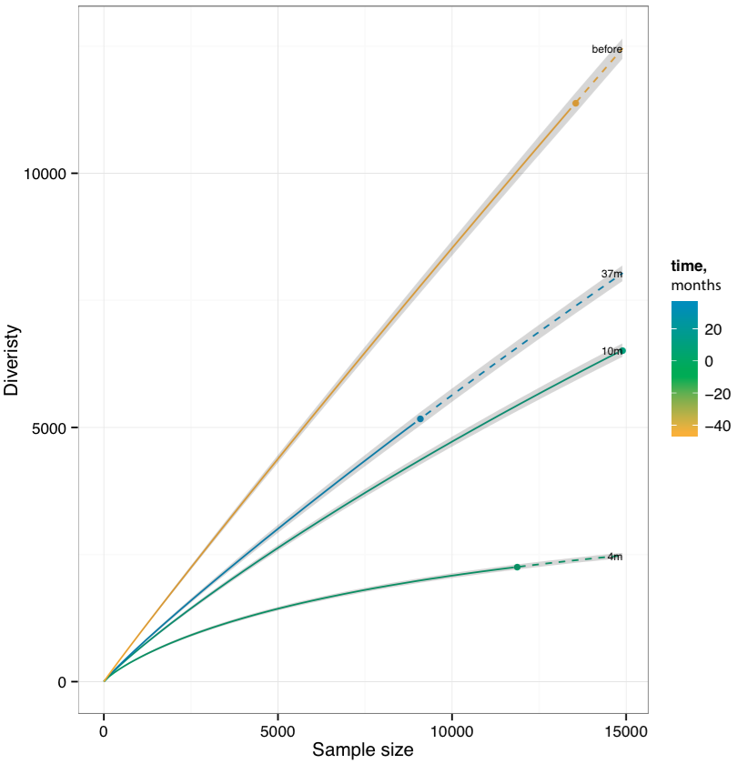
Rarefaction plot. Solid and dashed lines mark interpolated and extrapolated regions of rarefaction curves respectively, points mark exact sample size and diversity. Shaded areas mark 95% confidence intervals.
CalcDiversityStats
Computes a set of diversity statistics, including
- Observed diversity, the total number of clonotypes in a sample
- Lower bound total diversity (LBTD) estimates
- Chao estimate (denoted chao1)
- Efron-Thisted estimate
- Diversity indices
- Shannon-Wiener index. The exponent of clonotype frequency distribution entropy is returned.
- Normalized Shannon-Wiener index. Normalized (divided by
log[number of clonotypes]) entropy of clonotype frequency distribution. Note that plain entropy is returned, not its exponent. - Inverse Simpson index
- Extrapolated Chao diversity estimate, denoted chaoE here.
- The d50 index, a recently developed immune diversity estimate
Diversity estimates are computed in two modes: using original data and via several re-sampling steps (usually down-sampling to the size of smallest dataset).
- The estimates computed on original data could be biased by uneven
sampling depth (sample size), of those only
chaoEis properly normalized to be compared between samples. While not good for between-sample comparison, the LBTD estimates provided for original data are most useful for studying the fundamental properties of repertoires under study, i.e. to answer the question how large the repertoire diversity of an entire organism could be. - Estimates computed using re-sampling are useful for between-sample comparison, e.g. we have successfully used the re-sampled (normalized) observed diversity to measure the repertoire aging trends (see this paper).
Hint
In our recent experience the observed diversity and LBTD estimates computed on re-sampled data provide best results for between-sample comparisons.
Command line usage
java -Xmx4G -jar vdjtools.jar CalcDiversityStats \
[options] [sample1.txt sample2.txt ... if -m is not specified] output_prefix
Parameters:
| Shorthand | Long name | Argument | Description |
|---|---|---|---|
-m |
--metadata |
path | Path to metadata file. See Common parameters |
-i |
--intersect-type |
string | Set the intersection type used to collapse clonotypes before computing diversity. Defaults to strict (don’t collapse at all). See Common parameters |
-x |
--downsample-to |
integer | Set the sample size to interpolate the diversity estimates via resampling. Default = size of smallest sample. Applies to diversity estimates stored in .resampled.txt table |
-X |
--extrapolate-to |
integer | Set the sample size to extrapolate the diversity estimates. Default = size of largest sample. Currently, only applies to chaoE diversity estimate. |
--resample-trials |
integer | Number of resamples for corresponding estimator. Default = 3 | |
-h |
--help |
Display help message |
Tabular output
Two tables with diversity.[intersection type shorthand].txt and
diversity.[intersection type shorthand].resampled.txt are generated,
containing diversity estimates computed on original and down-sampled
datasets respectively.
Note that chaoE estimate is only present in the table generated for
original samples. Both tables contain means and standard deviations of
diversity estimates. Also note that standard deviation and mean values
for down-sampled datasets are computed based on N=3 re-samples.
Here is an example column layout, similar between both output tables:
| Column | Definition |
|---|---|
| sample_id | Sample unique identifier |
| … | Sample metadata columns, see Metadata section |
| reads | Number of reads in the sample |
| diversity | Diversity of the original sample (after collapsing to unique clonotypes according to -i parameter) |
| extrapolate_reads / resample_reads | The reads used to extrapolate or re-sample in order to compute present diversity estiamtes |
| <name>_mean | Mean value of the diversity estimate <name> |
| <name>_std | Standard deviation of the diversity estimate <name> |
| … |
Graphical output
none